Tensor descent: when and how to optimize in high dimensions?

• Introduction
• Tensor Muon?
  • Comparing TEON and tSVD-Muon
• References

Introduction

In [1], the authors proposed a brand new optimizer different from Adam-like optimizers, named Muon (Figure 1).

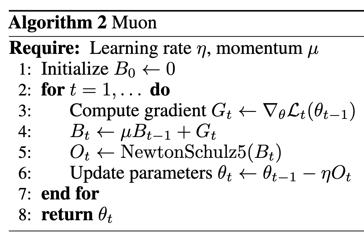
A key step is the NewtonSchulz5, which is an approximation of turning each of the singular value of the input matrix to 1.

def newtonschulz5(G, steps=5, eps=1e-7):
    assert G.ndim == 2
    a, b, c = (3.4445, -4.7750, 2.0315)
    X = G.bfloat16()
    X /= (X.norm() + eps)
    if G.size(0) > G.size(1):
        X = X.T
    for _ in range(steps):
        A = X @ X.T
        B = b * A + c * A @ A
        X = a * X + B @ X
    if G.size(0) > G.size(1):
        X = X.T
    return X

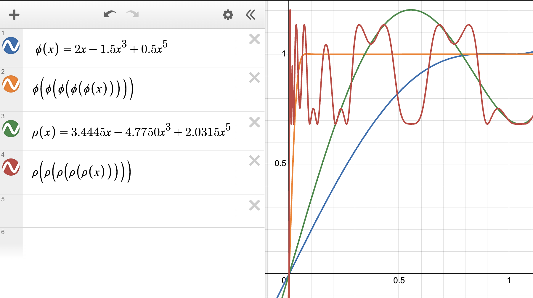
This NewtonSchulz is exactly applying the polynomial $p(x)=ax+bx^3+cx^5$ for five times on the input matrix signular values. The specific polynomial $(a, b, c) = (3.4445, -4.7750, 2.0315)$ looks as follows:

Tensor Muon?

A sudden idea came to me is that: Since we have multi-head attention, it seems to make more sense if we deal with each of the head as separate matrices, e.g. if $Q\in\mathbb{R}^{d\times d}$ with $Q = [Q_1,…,Q_{\text{num_head}}]$, we might want separate each $Q_i\in\mathbb{R}^{d\times d/\text{num_head}}$ as if they are a separate matrix. This idea is also backed by the new work [2], where they observe that separating the heads and conduct Muon separately seems to provide better performance.

A further thought becomes, essentially each head is playing a separate role as another dimension in the attention matrix, and we can stack each $Q_i$ in a new dimension to form a tensor $\mathcal{Q}\in \mathbb{R}^{d\times d/\text{num_head}\times \text{num_head}}$. How should I do Muon for this new tensor?

In [3], the authors proposed a tSVD method for third-order tensors that fits exactly in my purpose. The key idea is to define a tensor-tensor product $\ast$ via block-circulant structure: given $\mathcal{A}\in\mathbb{R}^{n_1\times n_2\times n_3}$ and $\mathcal{B}\in\mathbb{R}^{n_2\times \ell\times n_3}$, one takes the FFT along the third mode of both tensors, multiplies the corresponding frontal faces in the Fourier domain, and applies an inverse FFT. Under this product, one can define tensor transpose ($\mathcal{A}^T$ transposes each face and reverses faces $2$ through $n_3$), an identity tensor, and orthogonality ($\mathcal{Q}^T\ast\mathcal{Q}=\mathcal{I}$). The tSVD then decomposes $\mathcal{A}=\mathcal{U}\ast\mathcal{S}\ast\mathcal{V}^T$, where $\mathcal{U},\mathcal{V}$ are orthogonal tensors and $\mathcal{S}$ is f-diagonal (each frontal face is diagonal). In practice, this amounts to computing a standard matrix SVD for each frontal face in the Fourier domain, costing $O(n_1 n_2 n_3\log n_3 + n_3\cdot\text{SVD}(n_1, n_2))$.

Then, I read TEON [4] which did a different thing than I described above: instead of stacking heads within a layer, they stack gradients of the same type (Q with Q, K with K, V with V) from $K$ consecutive layers into a tensor $\mathcal{G}\in\mathbb{R}^{m\times n\times K}$, apply mode-1 matricization to get $M_1(\mathcal{G})\in\mathbb{R}^{m\times nK}$, orthogonalize this matrix, and fold back to update each layer. The mode choice is theoretically motivated: mode-1 is preferred when the top right singular vectors are aligned across layers. In practice, $K=2$ (stacking two neighboring layers) yields the best trade-off between capturing cross-layer correlations and maintaining singular vector alignment.

Comparing TEON and tSVD-Muon

Both TEON and the proposed tSVD-based approach stack layer gradients into a tensor, but they differ in how they orthogonalize. TEON flattens the tensor via matricization and orthogonalizes the resulting matrix, while tSVD-Muon works in the Fourier domain along the stacking dimension, applying per-face orthogonalization and coupling the faces through the FFT.

The key difference: TEON orthogonalizes one large $m\times nK$ matrix, coupling layers through column-concatenation. tSVD-Muon orthogonalizes $K$ separate $m\times n$ matrices in the Fourier domain, where the FFT/IFFT provides a different form of cross-layer coupling via circulant structure. When $K$ is small (e.g., 2), the FFT reduces to simple sums and differences of the faces, making tSVD-Muon easy to implement and interpret.

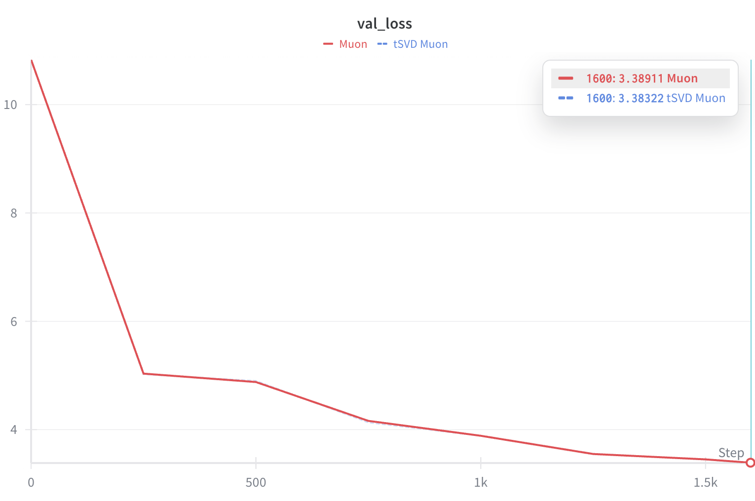
I didn’t have time to compare the tSVD-Muon with TEON in detail. Below I only incude a preliminary comparison of the proposed tSVD-Muon to the SOTA NorMuon implementation in the modded-nanogpt repo (I basically just made minimum changes over the NorMuon implementation in this file). The result is presented in Figure 3. Note that I did a small sweep over the learning rate for tSVD Muon.

The next questions are, 1. when is tensorized Muon better than the original Muon? 2. For big models, do we see an even bigger gain in performance or it get worse? To be continued…

References

1. K. Jordan et al., Muon: An optimizer for hidden layers in neural networks, webpost, 2024. ↑
2. T. Xie et al., Controlled LLM Training on Spectral Sphere, arXiv:2601, 2026. ↑
3. M. E. Kilmer, C. D. Martin, and L. Perrone, A Third-Order Generalization of the Matrix SVD as a Product of Third-Order Tensors, Tufts University, Department of Computer Science, Tech. Rep. TR-2008-4, 2008. ↑
4. R. Zhang et al., TEON: Tensorized Orthonormalization Beyond Layer-Wise Muon for Large Language Model Pre-Training, arXiv:2601.23261, 2026. ↑

If you find this post useful, you can cite it as:

@misc{li2026tensor,
  author = {Li, Jiaxiang},
  title  = {Tensor descent: when and how to optimize in high dimensions?},
  year   = {2026},
  url    = {https://jasonjiaxiangli.github.io/blog/tensor-muon/},
  note   = {Blog post}
}