Monotone Newton-Schulz: Near-Monotone Polynomial Iterations for Matrix Sign
Created: | Last modified:
NS iteration in Muon
In [1], the authors proposed a brand new optimizer different from Adam-like optimizers, named Muon (Figure 1).
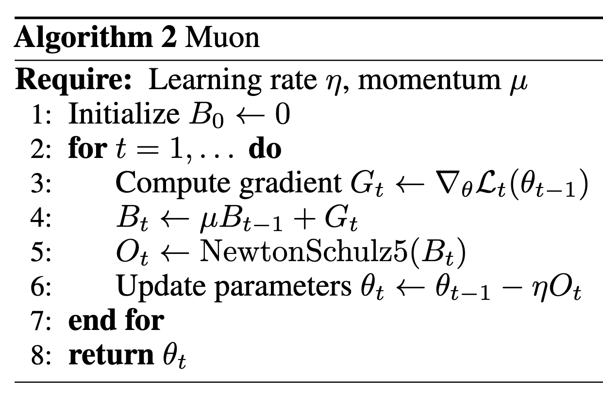
A key step of Muon is the NewtonSchulz5, which is an approximation of turning each singular value of the input matrix to 1.
def newtonschulz5(G, steps=5, eps=1e-7):
    assert G.ndim == 2
    a, b, c = (3.4445, -4.7750, 2.0315)
    X = G.bfloat16()
    X /= (X.norm() + eps)
    if G.size(0) > G.size(1):
        X = X.T
    for _ in range(steps):
        A = X @ X.T
        B = b * A + c * A @ A
        X = a * X + B @ X
    if G.size(0) > G.size(1):
        X = X.T
    return X
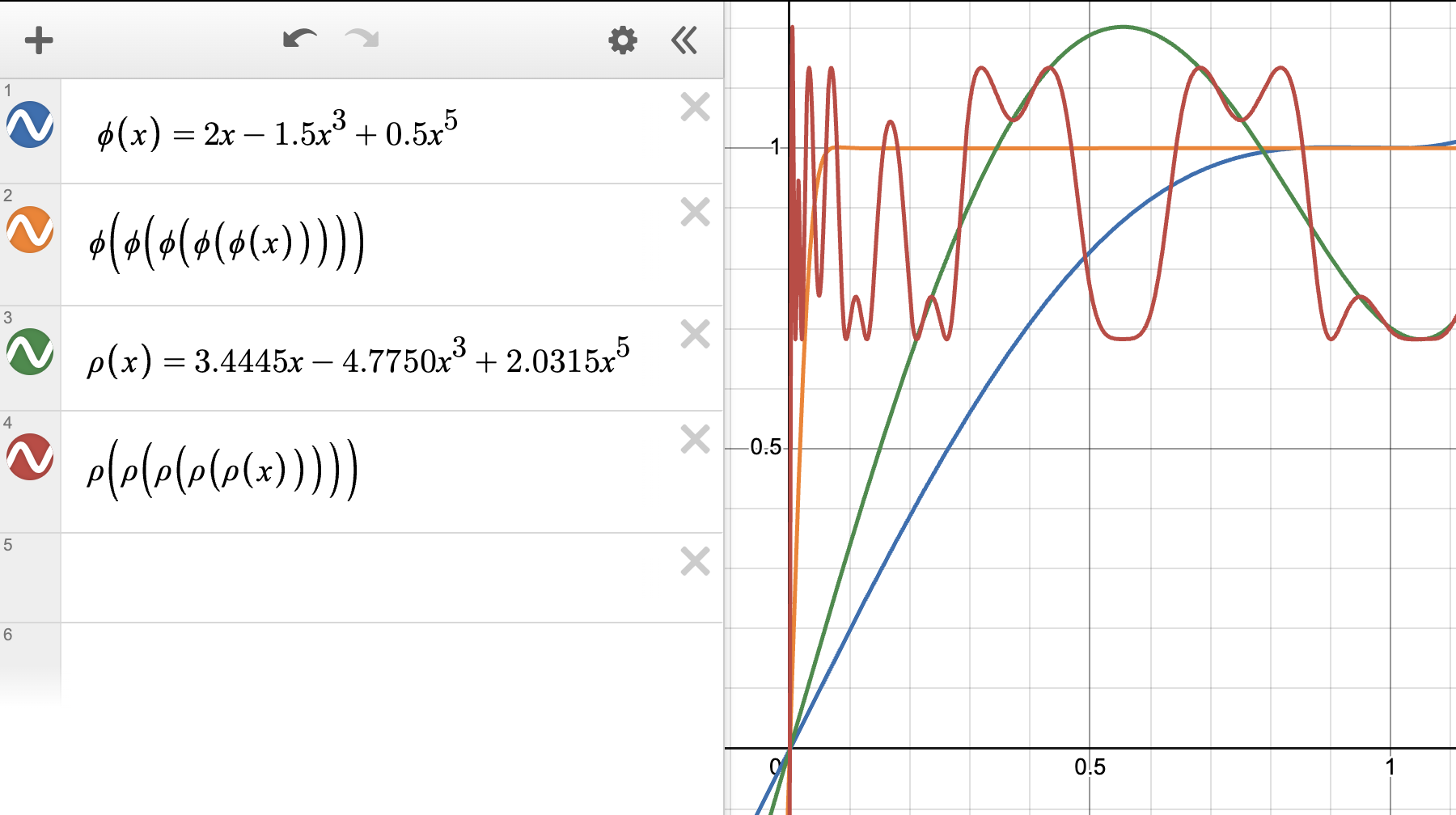
This NewtonSchulz is exactly applying the polynomial $p(x)=ax+bx^3+cx^5$ for five times on the input matrix. The specific polynomial $(a, b, c) = (3.4445, -4.7750, 2.0315)$ looks as follows:
A monotone NS step
However, after reading Prof. Su’s note [2], the steepest descent of each step really depends on the curvature function $H$ which controls the local Hessian landscape of the loss function. One interesting observation is that the optimal update direction may not have singular values strictly equal to 1, but is a direction that keeps the order of the spectrum of the gradient matrix while also making it more homogeneous (you can imagine it as uniformly squeezing all singular values toward 1, while still preserving their relative size/order).
In fact, as seen in the above figure, $(a, b, c) = (2, -1.5, 0.5)$ already satisfies this requirement, but it does not perform better than the default NS polynomial $(a, b, c) = (3.4445, -4.7750, 2.0315)$. The root cause might be that when $x$ is close to 0, $(a, b, c) = (2, -1.5, 0.5)$ does not bring the singular values to 1 as effectively as the default NS polynomial.
To this end, we wanna find a polynomial that is bringing the singular values to 1 as fast as he default NS polynomial, meanwhile still maintain the monotonicity. This is an approximation problem with certain constraints on the derivative of the polynomial: it should be always positive. To find such a polynomial, I directly solve for the optimal coefficients as a linear programming problem:
import numpy as np
from scipy.optimize import linprog

# ---- hyper-params (tweak these if needed) ----
delta = 1e-3     # contraction starts here (use 1e-3..1e-2)
alpha = 2.5      # lift strength
x0    = 0.01     # only lift on [0, x0]
eta   = 3e-1     # allow tiny negative slope on grid for robustness

# ---- grids ----
N  = 400
x  = np.linspace(0.0, 1.0, N)
xl = x[x <= x0]               # lift region
xc = x[x >= delta]            # contraction region

# variables: z = [a1, a2, a3, rho]
# objective: minimize rho
c = np.array([0.0, 0.0, 0.0, 1.0])

# Equality: p(1)=1  -> a1 + a2 + a3 = 1
Aeq = np.array([[1.0, 1.0, 1.0, 0.0]])
beq = np.array([1.0])

A = []
b = []

# 1) Monotone (approx): p'(x)=a1+3a2 x^2 + 5a3 x^4 >= -eta  ->  -(...) <= eta
for xi in x:
    A.append([-1.0, -3.0*xi**2, -5.0*xi**4, 0.0])
    b.append(eta)

# 2) Move toward 1 (no stalling): p(x) >= x  ->  -(a1 x + a2 x^3 + a3 x^5) <= -x
for xi in x:
    A.append([-xi, -xi**3, -xi**5, 0.0])
    b.append(-xi)

# 3) Gentle lift only on [0, x0]: p(x) >= alpha * x
if alpha > 0:
    for xi in xl:
        A.append([-xi, -xi**3, -xi**5, 0.0])
        b.append(-(xi * alpha))

# 4) Symmetric contraction on [delta,1]: |p(x)-1| <= rho(1-x)
#    p(x) - 1 <= rho(1-x)      ->  a1 x + a2 x^3 + a3 x^5 - (1-x) rho <= 1
#   -(p(x) - 1) <= rho(1-x)    -> -a1 x - a2 x^3 - a3 x^5 - (1-x) rho <= -1
for xi in xc:
    A.append([ xi,  xi**3,  xi**5, -(1.0 - xi)])
    b.append(1.0)
    A.append([-xi, -xi**3, -xi**5, -(1.0 - xi)])
    b.append(-1.0)

A = np.array(A, dtype=float)
b = np.array(b, dtype=float)

# bounds: a1,a2,a3 free; rho >= 0
bounds = [(None, None), (None, None), (None, None), (0.0, None)]

res = linprog(c, A_ub=A, b_ub=b, A_eq=Aeq, b_eq=beq, bounds=bounds, method="highs")
if not res.success:
    raise RuntimeError(f"LP failed: {res.message}")

a1, a2, a3, rho = res.x
print("a1,a2,a3 =", a1, a2, a3)
print("rho      =", rho)
print("a1+a2+a3 =", a1+a2+a3)

# quick checks
def pfun(xx): return a1*xx + a2*xx**3 + a3*xx**5
def compose(xx, k):
    yy = xx.copy()
    for _ in range(k): yy = pfun(yy)
    return yy

xx = np.linspace(0,1,2001)
pprime = a1 + 3*a2*xx**2 + 5*a3*xx**4
print("min p'(x) on grid:", float(np.min(pprime)))
y1 = pfun(xx)
y5 = compose(xx, 5)
mask = (xx >= delta) & (xx < 1.0)
print("max |p(x)-1| contraction check on [delta,1):",
      float(np.max(np.abs(y1[mask]-1) / (1-xx[mask]))))
print("max |1 - p^5(x)|:", float(np.max(np.abs(1 - y5[1:]))))
In above code, I discretized $[0,1]$ to 400 points and impose four constraints:
- monotonicity, $p’(x) \geq -\eta$ on $[0, 1]$;
- Progress toward 1, $p(x) \geq x$ on $[0, 1]$;
- Lift near 0, $p(x) \geq \alpha x$ on $[0, x_0]$;
- Contraction on $[\delta, 1]$, $\lvert p(x) - 1 \rvert \leq \rho(1-x)$
Running above code will output $(a1, a2, a3) = (2.625009142617934, -3.2408867395085266, 1.6158775968905927)$, and the plot of applying the polynomial five times looks like:
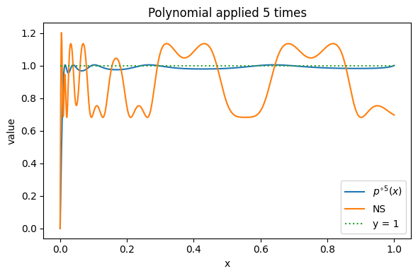
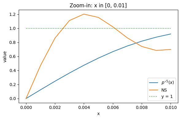
which seems to be a good alternative for the original polynomial coefficients. If we want a strict monotone polymonial, we can tune down $\alpha$ and $\eta$, but the Lift near 0 (condition 3) will be worse. In the experiments, I found that conditional 3 seems to be critical for a good training performance. However looking near 0, we can see that it’s still not as good as the default NS:
Therefore I turn to the method mentioned in Chebyshev approximation [3] and polar express [4]. In polar express paper [4], the authors propose to find not just one polynomial but a sequence of five different polynomials $p_1, \dots, p_5$ such that the composition $p_5 \circ p_4 \circ \cdots \circ p_1(x)$ approximates the constant function $y = 1$ on $[\ell, 1]$ far better than compositing one fixed polynomial five times.
The Polar Express approach
The key idea (Theorem 4.1 of [4]) is that the optimal composition can be found greedily: at each step $t$, solve a minimax problem
\[p_t = \arg\min_{p \in \mathbb{P}_5^{\text{odd}}} \max_{x \in [\ell_t, u_t]} |1 - p(x)|,\]then update the bounds as $\ell_{t+1} = \min_x p_t(x)$, $u_{t+1} = \max_x p_t(x)$ on $[\ell_t, u_t]$, and repeat. For numerical stability, a safety factor $p(x) \to p(x/1.01)$ and cushioning $\ell_{\text{eff}} = \max(\ell_t, u_t/10)$ are applied (Section 4.4 of [4]).
Adding near-monotonicity
The Polar Express polynomials are not monotone — the optimal first polynomial has $\min p’(x) \approx -6$. To obtain a near-monotone variant, I add two constraints to the minimax LP at each step:
- Near-monotonicity: $p’(x) \geq -\varepsilon$ on $[0, u_t]$, with $\varepsilon = 0.2$ (allowing a mild negative slope);
- Overshoot cap: $p(x) \leq 1.01$ on $[0, u_t]$, which prevents the upper bound $u_t$ from growing across compositions.
I also use empirical bound tracking — after applying each (safety-scaled) polynomial, the new $\ell_{t+1}, u_{t+1}$ are measured on a fine grid rather than using the formula $u_{t+1} = 2 - \ell_{t+1}$ from Theorem 4.1, which only holds for the unconstrained optimal polynomial.
The resulting LP, solved via cutting-plane refinement, is:
import numpy as np
from scipy.optimize import linprog

def solve_minimax_step(L, U, eps=0.2, cap=1.01, n_grid=500,
                       max_iter=15, refine_factor=4):
    """
    min_E  max_{x in [L,U]} |1 - p(x)|
    s.t. p'(x) >= -eps  on [0, U]   (near-monotonicity)
         p(x)  <= cap   on [0, U]   (tight overshoot control)
    where p(x) = a*x + b*x^3 + c*x^5.
    """
    pts_ap = np.linspace(L, U, n_grid)
    pts_gl = np.linspace(0, U, n_grid)

    for _ in range(max_iter):
        A_ub, b_ub = [], []
        for x in pts_ap:
            A_ub.append([ x,  x**3,  x**5, -1.0]); b_ub.append( 1.0)
            A_ub.append([-x, -x**3, -x**5, -1.0]); b_ub.append(-1.0)
        for x in pts_gl:
            A_ub.append([-1.0, -3*x**2, -5*x**4, 0.0]); b_ub.append(eps)
        for x in pts_gl:
            A_ub.append([x, x**3, x**5, 0.0]); b_ub.append(cap)

        res = linprog([0,0,0,1], A_ub=np.asarray(A_ub), b_ub=np.asarray(b_ub),
                      bounds=[(None,None)]*3+[(0,None)], method="highs")
        if not res.success:
            raise RuntimeError(f"LP: {res.message}")
        a, b, c, E = res.x

        # cutting-plane refinement on finer grid
        fine_ap = np.linspace(L, U, n_grid*refine_factor)
        fine_gl = np.linspace(0, U, n_grid*refine_factor)
        v_err = (np.abs(1-(a*fine_ap+b*fine_ap**3+c*fine_ap**5))-E).max()
        v_slp = (-(a+3*b*fine_gl**2+5*c*fine_gl**4)-eps).max()
        v_cap = (a*fine_gl+b*fine_gl**3+c*fine_gl**5 - cap).max()
        if max(v_err, v_slp, v_cap) <= 1e-6:
            return a, b, c, E
        if v_err > 1e-6:
            v = np.abs(1-(a*fine_ap+b*fine_ap**3+c*fine_ap**5))-E
            pts_ap = np.unique(np.append(pts_ap, fine_ap[np.argmax(v)]))
        if v_slp > 1e-6:
            v = -(a+3*b*fine_gl**2+5*c*fine_gl**4)-eps
            pts_gl = np.unique(np.append(pts_gl, fine_gl[np.argmax(v)]))
        if v_cap > 1e-6:
            v = a*fine_gl+b*fine_gl**3+c*fine_gl**5-cap
            pts_gl = np.unique(np.append(pts_gl, fine_gl[np.argmax(v)]))
    return a, b, c, E

def precompute_coeffs(T=5, ell=1e-3, eps=0.2, cap=1.01, safety=1.01):
    """Algorithm 2 with near-monotone constraint + empirical bound tracking."""
    ell_t, u_t = float(ell), 1.0
    coeffs = []
    for t in range(T):
        L = max(ell_t, u_t / 10.0)
        a, b, c, E = solve_minimax_step(L, u_t, eps=eps, cap=cap)
        if t < T - 1:
            a, b, c = a/safety, b/safety**3, c/safety**5
        coeffs.append((a, b, c, E))
        # empirical bound tracking
        fine = np.linspace(ell_t, u_t, 10000)
        vals = a*fine + b*fine**3 + c*fine**5
        ell_t, u_t = float(vals.min()), float(vals.max())
    return coeffs, ell_t, u_t
With $\varepsilon = 0.2$ and cap $= 1.01$, the five-step composition achieves $\max\lvert 1 - p^{\circ 5}(x)\rvert \approx 0.02$ for $x \geq 0.05$, while each individual polynomial has $\min p’(x) \geq -0.2$. I also compute a stricter variant (“Monotone PE $p\leq 1$”) with $\varepsilon = 0.01$ and cap $= 1.0$, which enforces near-strict monotonicity at the cost of slower convergence near $x = 0$.
Comparison
Figure 4 compares the five-fold composition of all four methods on $[0, 1]$:
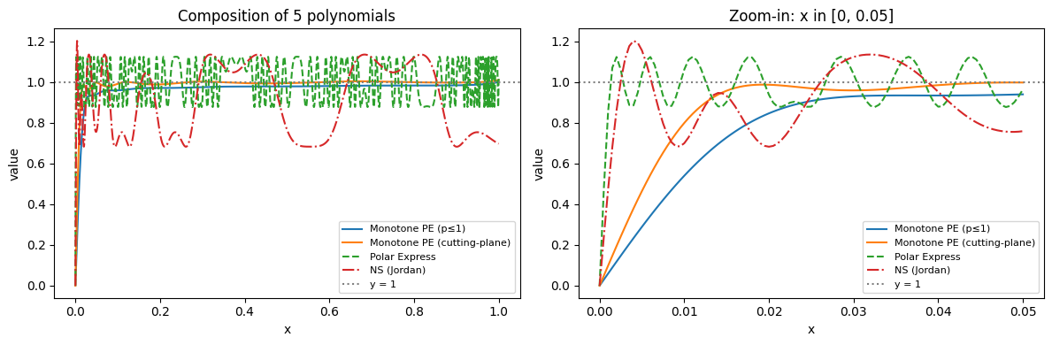
A few observations:
- Polar Express (green, dashed) converges fastest overall but oscillates significantly due to the non-monotone polynomials.
- NS (Jordan) (red, dash-dot) with the fixed polynomial $(3.4445, -4.7750, 2.0315)$ plateaus at $\approx 0.3$ error and does not converge.
- Monotone PE ($p \leq 1$) (blue) is the most conservative: strictly monotone but slower to lift small singular values.
- Monotone PE (cutting-plane) (orange) with $\varepsilon = 0.2$, cap $= 1.01$ strikes a balance: it stays within $\approx 2\%$ of $y = 1$ for $x \geq 0.05$ while maintaining near-monotonicity.
Numerical Experiments
I include a preliminary comparison of the proposed monotone NS (orange curve) against the Polar Express implementation in the modded-nanogpt repo. The result is presented in Figure 5 (note that I used the default hyperparameters; I also used two B200s with slight changes to the Triton kernels, so the val loss does not exactly match the reported 3.28 number).
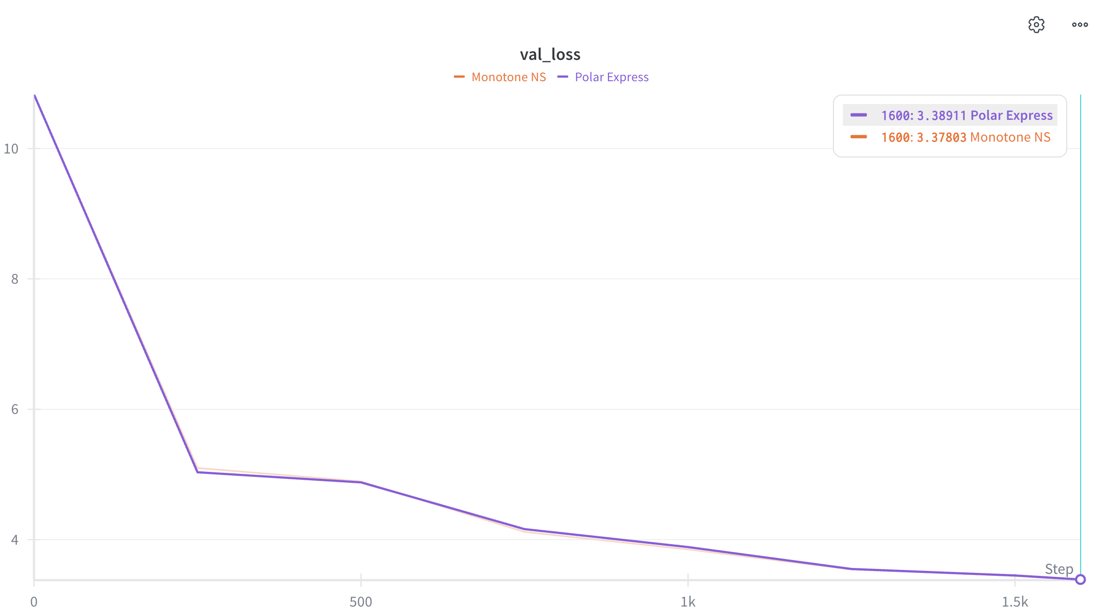
It is encouraging to see a slight advantage of monotone NS over Polar Express; however, this might simply be due to random seed variation. It remains to be seen whether this advantage holds in larger-scale experiments.
References
- K. Jordan et al., Muon: An optimizer for hidden layers in neural networks, webpost, 2024. ↑
- W. Su, Isotropic Curvature Model for Understanding Deep Learning Optimization: Is Gradient Orthogonalization Optimal?, arXiv:2511.00674, 2025. ↑
- E. Grishina, M. Smirnov, and M. Rakhuba, Accelerating Newton-Schulz Iteration for Orthogonalization via Chebyshev-type Polynomials, arXiv:2506.10935, 2025. ↑
- N. Amsel et al., The Polar Express: Optimal Matrix Sign Methods and Their Application to the Muon Algorithm, arXiv:2505.16932, 2025. ↑
If you find this post useful, you can cite it as:
@misc{li2026monotonens,
  author = {Li, Jiaxiang},
  title  = {Monotone Newton-Schulz: Near-Monotone Polynomial Iterations for Matrix Sign},
  year   = {2026},
  url    = {https://jasonjiaxiangli.github.io/blog/monotone-ns/},
  note   = {Blog post}
}